Customized Distributions • simstudy

Custom distributions can be specified in defData and defDataAdd by setting the argument dist to “custom”. When defining a custom distribution, you provide the name of the user-defined function as a string in the formula argument. The arguments of the custom function are listed in the variance argument, separated by commas and formatted as “arg_1 = val_form_1, arg_2 = val_form_2, $\dots$ , arg_K = val_form_K”.

Here, the arg_k’s represent the names of the arguments passed to the customized function, where $k$ ranges from $1$ to $K$ . You can use values or formulas for each val_form_k. If formulas are used, ensure that the variables have been previously generated. Double dot notation is available in specifying value_formula_k. One important requirement of the custom function is that the parameter list used to define the function must include an argument”n = n”, but do not include $n$ in the definition as part of defData or defDataAdd.

Example 1

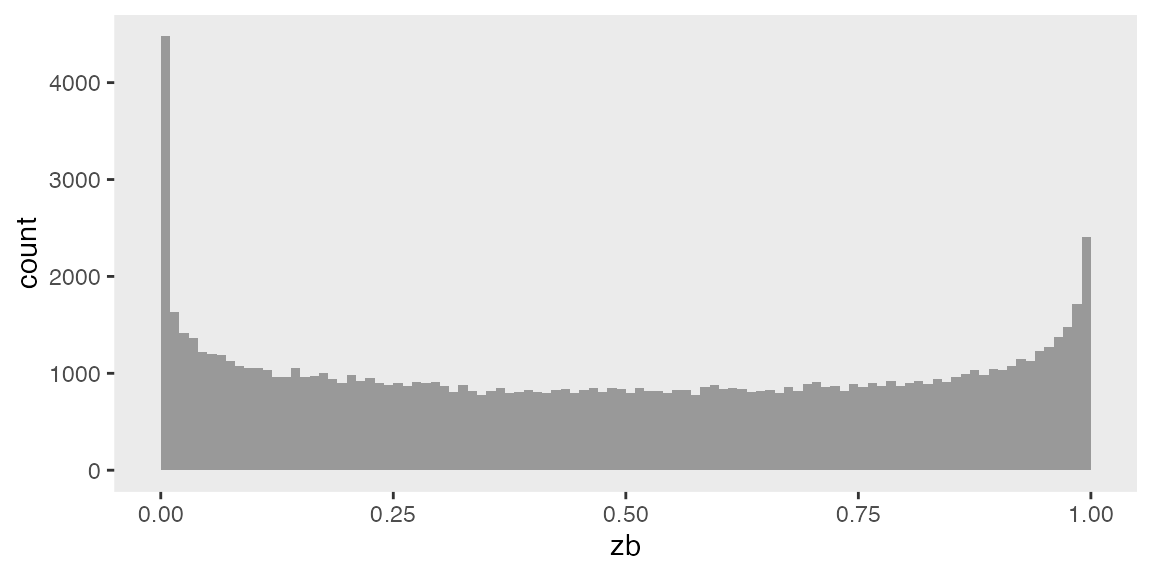
Here is an example where we would like to generate data from a zero-inflated beta distribution. In this case, there is a user-defined function zeroBeta that takes on shape parameters $a$ and $b$ , as well as $p_0$ , the proportion of the sample that is zero. Note that the function also takes an argument $n$ that will not to be be specified in the data definition; $n$ will represent the number of observations being generated:

zeroBeta <- function(n, a, b, p0) {
  betas <- rbeta(n, a, b)
  is.zero <- rbinom(n, 1, p0)
  betas*!(is.zero)
}

The data definition specifies a new variable $zb$ that sets $a$ and $b$ to 0.75, and $p_0 = 0.02$ :

def <- defData(
  varname = "zb", 
  formula = "zeroBeta", 
  variance = "a = 0.75, b = 0.75, p0 = 0.02", 
  dist = "custom"
)

The data are generated:

set.seed(1234)
dd <- genData(100000, def)

## Key: <id>
##             id         zb
##          <int>      <num>
##      1:      1 0.93922887
##      2:      2 0.35609519
##      3:      3 0.08087245
##      4:      4 0.99796758
##      5:      5 0.28481522
##     ---                  
##  99996:  99996 0.81740836
##  99997:  99997 0.98586333
##  99998:  99998 0.68770216
##  99999:  99999 0.45096868
## 100000: 100000 0.74101272

A plot of the data reveals dis-proportion of zero’s:

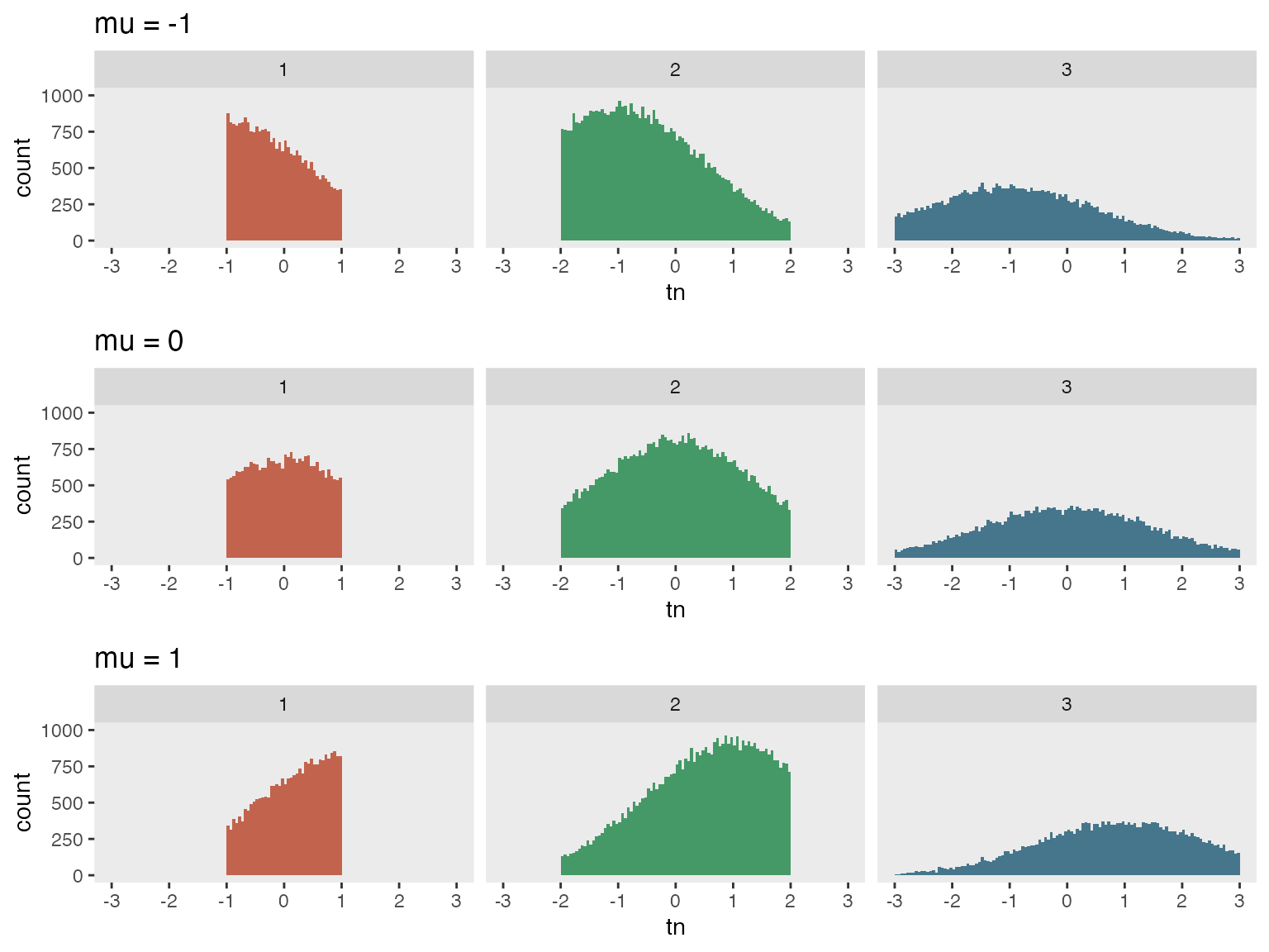
Example 2

In this second example, we are generating sets of truncated Gaussian distributions with means ranging from $-1$ to $1$ . The limits of the truncation vary across three different groups. rnormt is a customized (user-defined) function that generates the truncated Gaussiandata. The function requires four arguments (the left truncation value, the right truncation value, the distribution average and the standard deviation).

rnormt <- function(n, min, max, mu, s) {
  
  F.a <- pnorm(min, mean = mu, sd = s)
  F.b <- pnorm(max, mean = mu, sd = s)
  
  u <- runif(n, min = F.a, max = F.b)
  qnorm(u, mean = mu, sd = s)
  
}

In this example, truncation limits vary based on group membership. Initially, three groups are created, followed by the generation of truncated values. For Group 1, truncation occurs within the range of $-1$ to $1$ , for Group 2, it’s $-2$ to $2$ and for Group 3, it’s $-3$ to $3$ . We’ll generate three data sets, each with a distinct mean denoted by M, using the double-dot notation to implement these different means.

def <-
  defData(
    varname = "limit", 
    formula = "1/4;1/2;1/4",
    dist = "categorical"
  ) |>
  defData(
    varname = "tn", 
    formula = "rnormt", 
    variance = "min = -limit, max = limit, mu = ..M, s = 1.5",
    dist = "custom"
  )

The data generation requires three calls to genData. The output is a list of three data sets:

mus <- c(-1, 0, 1)
dd <-lapply(mus, function(M) genData(100000, def))

Here are the first six observations from each of the three data sets:

## [[1]]
## Key: <id>
##       id limit         tn
##    <int> <int>      <num>
## 1:     1     2  0.6949619
## 2:     2     2 -0.3641963
## 3:     3     2 -0.4721632
## 4:     4     3 -2.6083796
## 5:     5     2 -0.6800441
## 6:     6     3 -0.5813880
## 
## [[2]]
## Key: <id>
##       id limit         tn
##    <int> <int>      <num>
## 1:     1     1  0.4853614
## 2:     2     2 -0.5690811
## 3:     3     2  0.5282246
## 4:     4     2  0.1107778
## 5:     5     2 -0.3504309
## 6:     6     2  1.9439890
## 
## [[3]]
## Key: <id>
##       id limit         tn
##    <int> <int>      <num>
## 1:     1     2  1.3560628
## 2:     2     2  1.4543616
## 3:     3     3  1.4491010
## 4:     4     2  0.7328855
## 5:     5     2 -0.1254556
## 6:     6     2 -0.7455908

A plot highlights the group differences.